Probability density function | |||
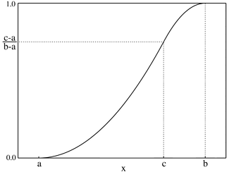
Cumulative distribution function | |||
| Parameters |
| ||
|---|---|---|---|
| Support | |||
| CDF | |||
| Mean | |||
| Median | |||
| Mode | |||
| Variance | |||
| Skewness | |||
| Excess kurtosis | |||
| Entropy | |||
| MGF | |||
| CF | |||
In probability theory and statistics, the triangular distribution is a continuous probability distribution with lower limit a, upper limit b, and mode c, where a < b and a ≤ c ≤ b.
Special cases
Mode at a bound
The distribution simplifies when c = a or c = b. For example, if a = 0, b = 1 and c = 1, then the PDF and CDF become:
Distribution of the absolute difference of two standard uniform variables
This distribution for a = 0, b = 1 and c = 0 is the distribution of X = |X1 − X2|, where X1, X2 are two independent random variables with standard uniform distribution.
Symmetric triangular distribution
The symmetric case arises when c = (a + b) / 2. In this case, an alternate form of the distribution function is:
Distribution of the mean of two standard uniform variables
This distribution for a = 0, b = 1 and c = 0.5—the mode (i.e., the peak) is exactly in the middle of the interval—corresponds to the distribution of the mean of two standard uniform variables, that is, the distribution of X = (X1 + X2) / 2, where X1, X2 are two independent random variables with standard uniform distribution in . It is the case of the Bates distribution for two variables.
Generating random variates
Given a random variate U drawn from the uniform distribution in the interval (0, 1), then the variate
where , has a triangular distribution with parameters and . This can be obtained from the cumulative distribution function.
Use of the distribution
See also: Three-point estimationThe triangular distribution is typically used as a subjective description of a population for which there is only limited sample data, and especially in cases where the relationship between variables is known but data is scarce (possibly because of the high cost of collection). It is based on a knowledge of the minimum and maximum and an "inspired guess" as to the modal value. For these reasons, the triangle distribution has been called a "lack of knowledge" distribution.
Business simulations
The triangular distribution is therefore often used in business decision making, particularly in simulations. Generally, when not much is known about the distribution of an outcome (say, only its smallest and largest values), it is possible to use the uniform distribution. But if the most likely outcome is also known, then the outcome can be simulated by a triangular distribution. See for example under corporate finance.
Project management
The triangular distribution, along with the PERT distribution, is also widely used in project management (as an input into PERT and hence critical path method (CPM)) to model events which take place within an interval defined by a minimum and maximum value.
Audio dithering
The symmetric triangular distribution is commonly used in audio dithering, where it is called TPDF (triangular probability density function).
See also
- Trapezoidal distribution
- Thomas Simpson
- Three-point estimation
- Five-number summary
- Seven-number summary
- Triangular function
- Central limit theorem — The triangle distribution often occurs as a result of adding two uniform random variables together. In other words, the triangle distribution is often (not always) the result of the first iteration of the central limit theorem summing process (i.e. ). In this sense, the triangle distribution can occasionally occur naturally. If this process of summing together more random variables continues (i.e. ), then the distribution will become increasingly bell-shaped.
- Irwin–Hall distribution — Using an Irwin–Hall distribution is an easy way to generate a triangle distribution.
- Bates distribution — Similar to the Irwin–Hall distribution, but with the values rescaled back into the 0 to 1 range. Useful for computation of a triangle distribution which can subsequently be rescaled and shifted to create other triangle distributions outside of the 0 to 1 range.
References
- Kotz, Samuel; Dorp, Johan Rene Van (2004-12-08). Beyond Beta: Other Continuous Families Of Distributions With Bounded Support And Applications. World Scientific. ISBN 978-981-4481-24-3.
- "Archived copy" (PDF). www.asianscientist.com. Archived from the original (PDF) on 7 April 2014. Retrieved 12 January 2022.
{{cite web}}: CS1 maint: archived copy as title (link) - "Archived copy" (PDF). Archived from the original (PDF) on 2006-09-23. Retrieved 2006-09-23.
{{cite web}}: CS1 maint: archived copy as title (link)
External links
- Weisstein, Eric W. "Triangular Distribution". MathWorld.
- Triangle Distribution, decisionsciences.org
- Triangular Distribution, brighton-webs.co.uk
- Proof for the variance of triangular distribution, math.stackexchange.com


 , has a triangular distribution with parameters
  and
and  . This can be obtained from the cumulative distribution function.
 ). In this sense, the triangle distribution can occasionally occur naturally. If this process of summing together more random variables continues (i.e.
  ), then the distribution will become increasingly bell-shaped.